Where a distribution puts its probability

Three probaverse packages went to CRAN this week. Behind them is one idea, and one new verb.

• distionary 0.2.0 — a distribution now says where it keeps its probability.
• distplyr 0.3.0 — every verb understands that.
• probaverse 0.1.1 — installs the matching set.

The idea

Probability comes in two forms. Some of it sits on single points. Some of it is spread over a range.

A distribution used to know only how to answer questions. Now it also knows which of those two forms it is made of, and where. That record is called its support. The single points are called atoms.

A Poisson distribution keeps its probability on 0, 1, 2, and so on:

library(probaverse)
support(dst_pois(3))

## <support: discrete>
## -- atoms --
## Integer series of length Inf:
## 0, 1, 2, 3, 4, 5, ...

That list is not cut off at some large number. It is the whole infinite set, handled by the discretes package.

Why it matters

A distribution can have both forms at once. Take rainfall: no rain on 40% of days, and an exponential amount on the rest.

rain <- mix(dst_degenerate(0), dst_exp(rate = 0.2), weights = c(0.4, 0.6))
support(rain)

## <support: mixed>
## -- atoms --
## Numeric vector series of length 1:
## 0
## -- continuous --
## [0, Inf]

One atom, sitting on zero. Then a range above it.

Now ask for some quantiles. Four days in ten are dry, so anything up to 0.4 should come back as exactly zero:

eval_quantile(rain, at = c(0.3, 0.4, 0.5))

## [1] 0.0000000 0.0000000 0.9116078

Exactly zero, not nearly zero. That is the part that used to be hard. Without a support, the package assumed probability was spread smoothly, so it went looking for the place where the curve crossed 0.4. There is no such place. The curve jumps straight over it.

The graft

The simplest way to turn data into a distribution is to use the data itself, giving every observation an equal share. This is sometimes called Historical Simulation.

Here are a hundred years of Nile flows:

flows <- dst_empirical(Nile)
vtype(flows)

## [1] "discrete"

Discrete: one atom per observation.

Now ask it about a flood so rare it shows up once in a thousand years:

eval_quantile(flows, at = 0.999)

## [1] 1370

That is simply the largest flood on record. The data has nowhere else to put one.

So make a second piece to cover the part the record cannot. Take the floods above 1150, and fit a generalised Pareto to how far each one exceeded it, using famish:

u <- 1150
tail_fit <- fit_dst_gp(Nile[Nile > u] - u)
tail_fit

## Generalised Pareto distribution (continuous) 
## --Parameters--
##      scale      shape 
## 75.0231325 -0.1522667

Two pieces now: the record, and a model for its top end. graft_right() stitches them together at 1150.

flood <- graft_right(flows, of = u, tail_excess = tail_fit)
flood

## Graft distribution (mixed)
## --Components--
##  distribution                           weight
##  Finite                                 0.88  
##  Shifted(Generalised Pareto(75, -0.15)) 0.12

The support shows both halves:

support(flood)

## <support: mixed>
## -- atoms --
## Numeric vector series of length 76:
## 456, 649, 676, ..., 1120, 1140, 1150
## -- continuous --
## [1150, 1642.71]

eval_quantile(flood, at = c(0.99, 0.999))

## [1] 1305.214 1405.025

The atoms are the observations that survived the cut. The range after them is the fitted tail. That tail came out bounded, so the support also tells you where it stops.

And the thousand-year flood is now a number the record never contained.

It is easier to see on the survival function, which plots the chance of exceeding each flow. The record runs out at its largest value and simply stops. The graft carries on past it.

plot(flood, "survival", from = 456, to = 1500, n = 8001, log = "y",
     ylim = c(1e-3, 1), col = "red", lty = 2, lwd = 2,
     xlab = "Annual flow", ylab = "Chance of exceeding")
plot(flows, "survival", from = 456, to = 1500, n = 8001, add = TRUE, lwd = 2)
abline(v = u, col = "grey60", lty = 3)
text(u, 1e-3, " graft point", col = "grey40", adj = c(0, 0), cex = 0.8)
legend("bottomleft", legend = c("the record alone", "with a grafted tail"),
       col = c("black", "red"), lty = c(1, 2), lwd = 2, bty = "n")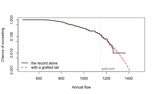

One install

A good idea in one package is a breaking change in the others. distplyr 0.3.0 needs distionary 0.2.0. So probaverse 0.1.1 now records minimum versions for the packages it loads.

install.packages("probaverse")

A mixed-up library comes back up to a set that works together.

What’s next

When distionary went to CRAN, I said that proper support for discrete and mixed distributions was coming. This is it, by way of a package about infinite sets.

Real data is lumpy. Flows that are sometimes zero, records made of nothing but discrete points. The probaverse could always describe these. Now it can compute with them.

Next: multivariate distributions, and families of distributions rather than single ones.