Introducing probaverse 0.1.0

It wasn’t supposed to be a “-verse”. I just needed to be able to manipulate some probability distributions. But then three clearly different tasks needed special handling.

• I needed to define the distribution object in the first place. Out came distionary.
• Manipulation of these distributions could then be handled by distplyr.
• The need to fit and tune distributions to data quickly followed, and so did famish.

And, to tie them all together, probaverse. If you’re familiar with how the tidyverse package loads the core tidyverse packages, probaverse is similar: it’s a meta-package whose purpose is simply to load… well, the probaverse packages.

So, all you have to do is

library(probaverse)

## ── Attaching core probaverse packages ──────────────────────────────────────────
## ✔ distionary   0.1.0   Create and Evaluate Probability Distributions
## ✔ distplyr     0.2.0   Manipulate and Combine Probability Distributions
## ✔ famish       0.2.0   Flexibly Tune Families of Probability Distributions

…and the whole suite is loaded.

That one call matters because the packages underneath are meant to feel like one toolkit.

If you can’t tell, probaverse takes inspiration from tidyverse. Aside from the obvious similarities in some of the package names (tidyverse → probaverse, dplyr → distplyr), probaverse also strives to follow the tidyverse design principles.

It shares the four guiding principles of being human centered, consistent (between packages), composable (between parts), and inclusive (to diverse groups of people).

For example, take the waiting times between eruptions from the built-in faithful data frame:

x <- faithful$waiting

We can use distionary to create an empirical (data-based) distribution, and famish to fit a gamma distribution to the data.

d1 <- dst_empirical(x)
d2 <- fit_dst_gamma(x)

## Loading required namespace: testthat

Watching Old Faithful through six successive eruptions gives five inter-eruption waiting times; the shortest among them is the minimum of five draws from the model. In distplyr, minimize(..., draws = 5) is the distribution of that quantity.

m1 <- minimize(d1, draws = 5)
m2 <- minimize(d2, draws = 5)

You can calculate the quartiles to get a sense of the inter-quartile range and the median.

enframe_quantile(m1, m2, at = c(0.25, 0.50, 0.75))

## # A tibble: 3 × 3
##    .arg quantile_m1 quantile_m2
##   <dbl>       <dbl>       <dbl>
## 1  0.25          48        49.9
## 2  0.5           52        55.3
## 3  0.75          57        60.6

Or just get the means:

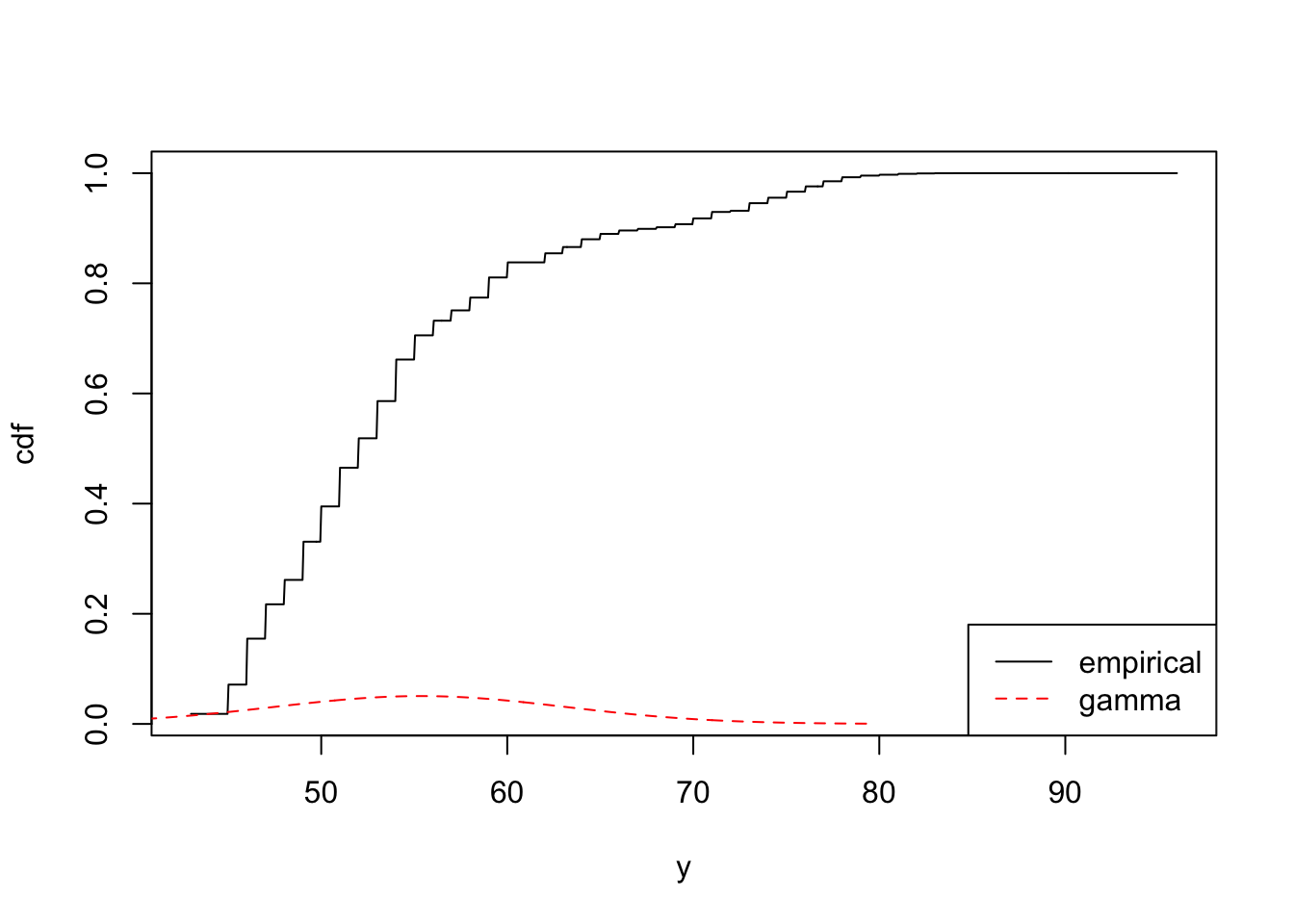
mean(m1)

## [1] 54.16665

mean(m2)

## [1] 55.27021

Check out a quick plot comparing the CDF of both models.

plot(m1, n = 1000)
plot(m2, add = TRUE, n = 1000, col = "red", lty = 2)
legend(
  "bottomright",
  legend = c("empirical", "gamma"),
  col = c("black", "red"),
  lty = c(1, 2)
)

This is a simple example, but you can go much further with the suite: fitting, evaluating, and transforming distributions, among other workflows. Some of these will be featured in future blog posts. Consider, for example, using it to fit a probabilistic machine learning model.

Currently, probaverse focuses on univariate distributions. The roadmap includes multivariate distributions (including construction via copulas), richer tooling for empirical distributions such as kernel density estimation, and user-defined parametric families so custom models can be specified and fitted alongside built-in choices like Normal, Poisson, and Gumbel.